Exponentially Weighted Average and Momentum
2021-01-04 Intro , Exponentially Weighted Average added
This article will discuss Exponentially Weighted Average and Momentum. Exponentially Weighted Average provides a solution that can solve the problem of stochastic gradient with only the gradient for each step. I reviewed it again and wrote it as a Closed Book 3 days later.
Exponentially Weighted Average
DLS describes Exponentially Weighted Average as an example of calculating the average rainfall for the city of London.


The statistical significance of this is that V is an average that roughly reflects the number of \(1 \over {1-\beta}\). For example, if \(\beta\) is 0.9, then V reflects the weather for 10 days.
Therefore, as \(\beta\) increases, the graph becomes smooth, while as \(\beta\) decreases, the number of reflected days decreases, showing a rapidly changing graph.
Weighted Average in statistical view
f we expand the above expression
\[V_n = {\beta}^n (1-\beta) \theta_0 +{\beta}^{n-1} (1 - \beta ) \theta_{1} + .. + (1 - \beta ) \theta_{n}\]it’ the result.

There are some exponentially decreasing graphs. The exponentially weighted average is the sum of the weather values multiplied by element wise.
And, Professor Andrew explains the reason for the average that roughly reflects the number of \(1 \over {1-\beta}\),
Since \((1 - \epsilon) ^{1 \over \epsilon} = {1 \over e }\) , it is said to reflect the latest data as much as \({1-\beta}\). I’ve also tried calculating the geometric series, and a ratio of about 0.7 comes out, and the professor says it’s the rule of thumb, but for now, I decided to just accept it.
To do the calculation, we would compute the expression ,\(\sum_{k=1}^{10} = { (1- \beta) \beta^{k-1}}\). The data reflection ratio of the latest 10 temperatures is about 0.7. This is true even if it becomes \(n \to \infty\) . I think you expressed it that way because you used the expression rule of thumb empirically because it reflected the amount of data as much as \(1 \over {1-\beta}\)
Assuming that the total number of weather is infinite, the desired interested ratio can be obtained instead of simply having a interested ratio of 0.7.
Suppose we show that avearge is the avearge of the 1 .. k th term.
\[\alpha [ {(1-\alpha) }^k + {(1-\alpha) }^{k+1} + {(1-\alpha) }^{k +2} ... ]\]The above will not be interseted term.
\[\alpha {(1-\alpha) }^k [1 + {(1-\alpha) }^1 + {(1-\alpha) }^2 ... ]\]The above term can be written like this:
\[{weighted \ omitted \ by \ stopping \ after\ k \ terms \over \ total \ weight}\] \[= { \alpha [ {(1-\alpha) }^k + {(1-\alpha) }^{k+1} + {(1-\alpha) }^{k +2} ... ] \over {\alpha (1-\alpha) }^k [1 + {(1-\alpha) }^1 + {(1-\alpha) }^2 ... ] }\] \[= { \alpha {(1-\alpha) }^k \over {1 \over {1 - (1-\alpha )}} }\] \[= {(1-\alpha) }^k\]Therefore, formulating how many terms are excluded from the total can be expressed as above. For example, let’s make the k-th term reflect 99% of the time. \(0.01 = {(1-\alpha) }^k\) \(k = {\ln (0.01)} \over {\ln (1-\alpha)}\) will be The Taylor series says that \(\alpha \to 0 \ as \ N \to \inf\) gives \(\ln { (1-alpha) } \to {- \alpha }\) .
\[k \approx { {\ln (0.01)} \over {- \alpha} }\]You will get the relation When \(\alpha = 0 .1\) , it is possible to reflect 90 percent of the approximate 23 terms. (If there is something in the description that is not correct, please leave a comment or an email.)
Gradient Descent Momentum

Update proceeds through the same rule as above.
Professor Andrew
You said that it is similar to the law of physics, where friction is applied to the existing running speed (dV) and (\(\beta\) ) is accelerated as much as the force is applied ( \((1 - \beta ) dW\)).
Comparing Weighted Average and Gradient Descent, Gradient Descent udpates the weight with only the instantaneous gradient.
Therefore, gradient descent changes direction more abruptly, but momentum does not change direction abruptly because momentum advances while maintaining its direction according to acceleration. To put this in terms, gradient descent is prone to influence when bad values are calculated due to variance of Hessian matrix and stochastic (mini-batch gradient descent). However, momentum reflects the value of the existing Hessian matrix and the value of the existing data, so it is less affected when a bad value is calculated.

I was able to see that this expression was used in various sources with different expressions. In the above two photos, v is in the same direction as the gradient,
The two photos below were taken in the opposite direction of the gradient (the direction of the minimum). However, using the concepts of the theory of velocity and acceleration in physics does not change.
I know momentum is fast, but I didn’t say exactly how fast it gets. We will prove this using mathematics and physics.
In conclusion, compared to stochastic gradient descent, it is faster by \({1 \over (1-\beta) }\).
And, if the gradient is constant, v does not increase further when the gradient and the friction force ((1-\(\beta\))v) are equal. This is called the terminal velocity.
\[friction - accel = 0\] \[(1-\beta)v = \epsilon d \theta\] \[v = \epsilon {1 \over (1-\beta) } d \theta\]For example, if \(\alpha (or \beta)\) is 0.9, then the terminal velocity is 10 times the gradient, which is about 10 times faster than the stochastic gradeint descent.
omit learning rate
\[dV = \beta dV + \alpha dW\] \[W = : W - \alpha dV\]It is said that the use of the above expression by omitting the learning rate is also shown in the paper. Even in the deeplearning book, I know that the learning rate is explained by omitting the weight udpate. There is no detailed explanation for this, but here are my thoughts:
\[dV = \beta dV + dW\] \[\alpha dV = \alpha \beta dV + \alpha dW\] \[dV \approx \alpha \beta dV + \alpha dW\] \[W = : W - dV\](I’m not sure. If anyone knows, please let me know in the comments or e-mail.)
why use viscous drag ?
What I’m going to say from now on may be uncomfortable to read. Feel free to skip it. I tried to write it as simply as possible. (If the explanation is not accurate, please let me know in the comments or by e-mail.)
You understand that both acceleration and friction exist. From now on, the word frictional force will be used interchangeably with drag force, but it has the same meaning. This time, it is an explanation of the types of drag of . There are many types of drag forces in the world. There are dry friction , viscous drag , turbulent drag .. and so on. The drag we use here is the drag viscous drag proportional to v. If so, these questions may arise.
Why did you have to use viscous drag? Shouldn’t dry friction and turbulent drag be used?
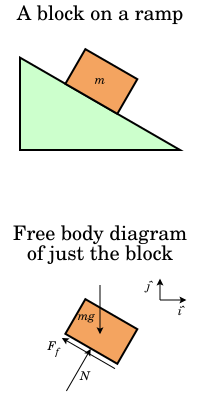
A simple explanation of dry friction is that a fixed force is applied. For example, an object of mass m standing on a slope has a frictional force proportional to its gravity (constant).
Viscous drag is applied with drag (force) proportional to speed. Turbulent drag is the applied drag (force) proportional to the square of v.
\[v := v - c\]Because dry friction always applies a fixed force to the particle, the particle will never reach the local minima at \(\theta\) and the velocity will be zero.
When viscous drag works 


The top picture is the time/velocity graph of turbulent drag, and the bottom graph is the height/distance graph of viscous drag. I brought the above photos for conceptual understanding rather than an accurate explanation. Each, assuming that only drag acts, in the case of turbulent drag, it can be seen that the speed is kept constant, and in the case of viscous drag, the speed becomes 0 during stroke movement, and it rises to a certain height and then goes down again.
In summary, dry friction can be so extremely slow that it cannot reach the local minma. In the case of turbulent drag, the velocity is never zero, so adding a gradient to it will always move away from the starting point at a velocity of \(O( \log t)\) forever. If viscous drag is used to solve these extreme properties, the local minima can be reached because the drag is not as strong as the dry friction, and the speed can be reduced if the direction of the gradient is not the direction to be minimized.
implementation in deep learning

If the above expression is applied as it is when implementing the actual implementation, the initial value will be smaller than the expected value because \(V_0 = 0\) is initialized and started. Therefore, scaling is performed by dividing by \(1 \over 1 - {\beta}^t\). As t increases, the scaling factor approaches 1. This is because the weighted average reflects the latest data as many as \(1 \over {1-\beta}\) .
gradient descent vs gradient decent momentum
You can use gradient descent to reflect the latest data like momentum. For example, if \(\beta\) is 0.99, you can put gradients for 100 data in memory. However, momentum can solve this with one line of code. Although statistics are not essential, I felt that it could be a good tool in advancing algorithms.
Reference
| [1] [Improving Deep Neural Networks: Hyperparameter Tuning, Regularization and Optimization - 홈 | Coursera](https://www.coursera.org/learn/deep-neural-network/home/welcome) |
Leave a comment